Embedding Molecules into a Latent Space
As mentioned in my previous post on predicting bee toxicity, it is often necessary to convert heterogeneous molecular structures into latent-space representations to allow machine learning methods to identify predictive features. After publishing the bee toxicity paper, a potential collaborator (hi Vasuk!) sent over a data set, asking if we might be able to apply a similar method to extract meaningful structure-activity relationships.
The data are the interactions of 49 common small molecules present in cannabis–loosely, a selection of cannabinoids and terpenoids–and their interactions with a host of receptor proteins (including cannabinoid receptors, adrenergic receptors, and ion channels):
| Compound Name | Structure | Protein Affinities |
|---|---|---|
| Δ-9 Tetrahydrocannabinol | 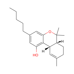 |
PGH Synthase 1, CB-1, CB-2 |
| Cannabigerol | 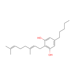 |
CB-1, CB-2, α-2A, α-2B, 5-HT 1A |
| … | … | … |
| Cannabidiol-C4 | 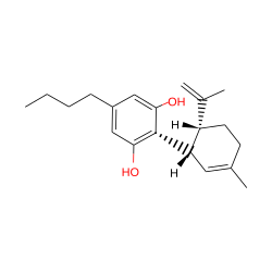 |
None |
As with the bee toxicity study, the first step (after cleaning and pre-processing the raw data) has to be taking these molecules–handily provided as SMILES strings–and making pairwise comparisons via a graph kernel. To do this, I used a piece of software I’ve been developing: MolecularGraphKernels.jl. The software provides a handy interface for taking molecular structure encodings and applying various graph kernels, plus some useful visualization and other utilities. This is still in active development (read: the codebase is highly unstable and will change frequently in the near future) but I look forward to making a full post on it when we hit our first stable release.
Like with my PoreMatMod.jl software, MolecularGraphKernels.jl is intended to be streamlined and straightforward, for use by scientists of any (or no) familiarity with coding and computational chemistry. Given data like we have above, generating the pairwise (Gram) kernel score matrix is as easy as:
# turn the SMILES into graphs
using MolecularGraph #¹
using MolecularGraphKernels
graphs = MetaGraph.(smilestomol.(data.smiles))

# calculate Gram matrix
gmat = gram_matrix(random_walk, graphs; l=4, normalize=true)
¹ MolecularGraph.jl by Seiji Matsuoka
From here, to convert the data from 49-dimensional space into something a bit more human-accessible, we need to apply a dimensional reduction technique. There are many to choose from, but for this demo we’ll apply diffusion mapping:
# apply diffusion mapping to 2 dimensions
using DiffusionMap #²
normalize_to_stochastic_matrix!(gmat)
mapped = diffusion_map(gmat, 2)Now that everything is transformed into a two-dimensional space, we can check the embedding out visually:
Looks like we do get some separation of the bio-active vs. inactive substances, which is pretty neat, since we never told the model about these classifications ahead of time–we only colored the points in the latent space after the fact. Looking at the structures for the local clusterings of points (hover the mouse cursor to get a tooltip with the line drawing) we can also see that related molecules tend to bunch together. Not bad for a first pass on the data!